Spreadsheets

Formulas

The same formulas you use in Excel. SUM, VLOOKUP, IF — they all work here.

How Formulas Work

Type = then your calculation. You can add cells, use functions, or do math.


=A1+B1           Add two cells
=SUM(A1:A10)     Add up a range
=(A1+B1)*C1      Use parentheses for order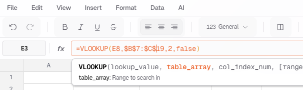

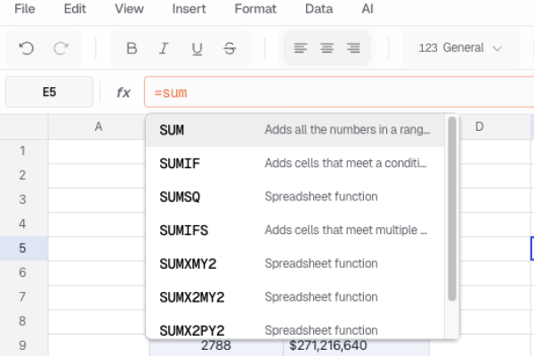
Formula bar showing a VLOOKUP formula — The formula bar shows your formula with hints for each parameter

Tip

Start typing a function name and press Tab to autocomplete it.

Formula autocomplete dropdown — Suggestions appear as you type, with descriptions for each function

Cell References

The Basics

Reference	What it means	Example
`A1`	One cell	`=A1*2`
`A1:B10`	A range of cells	`=SUM(A1:B10)`
`A:A`	A whole column	`=SUM(A:A)`
`1:1`	A whole row	`=SUM(1:1)`

Relative vs Absolute

When you copy a formula, references change by default. Add $ to lock a row or column.

Type	Syntax	When you copy it…
Relative	`A1`	Changes to match the new position
Lock column	`$A1`	Column stays A, row changes
Lock row	`A$1`	Row stays 1, column changes
Lock both	`$A$1`	Never changes

Tip

Press F4 while editing a reference to cycle through these options.

Referencing Other Sheets

Use the sheet name followed by ! to pull data from another sheet:


=Sheet2!A1                  One cell from Sheet2
=SUM(Sheet2!A1:A10)         A range from Sheet2
='Sales Data'!B5            Sheet name with spaces needs quotes

All Formulas by Category

Math & Statistics

Formula	What it does	Example
`SUM`	Add numbers	`=SUM(A1:A10)`
`AVERAGE`	Get the average	`=AVERAGE(B1:B100)`
`COUNT`	Count numbers	`=COUNT(A:A)`
`COUNTA`	Count non-empty cells	`=COUNTA(A:A)`
`MIN`	Find the smallest	`=MIN(A1:A100)`
`MAX`	Find the largest	`=MAX(A1:A100)`
`ROUND`	Round to X decimals	`=ROUND(A1, 2)`
`ABS`	Remove negative sign	`=ABS(A1)`
`SQRT`	Square root	`=SQRT(A1)`
`POWER`	Raise to a power	`=POWER(A1, 2)`
`MEDIAN`	Find the middle value	`=MEDIAN(A1:A100)`
`STDEV`	Standard deviation	`=STDEV(A1:A100)`

Lookup & Reference

Formula	What it does	Example
`VLOOKUP`	Look up a value in a table	`=VLOOKUP(A1, B:C, 2, FALSE)`
`HLOOKUP`	Look up horizontally	`=HLOOKUP(A1, 1:2, 2, FALSE)`
`INDEX`	Get cell at row/column	`=INDEX(A1:C10, 2, 3)`
`MATCH`	Find position of a value	`=MATCH(A1, B:B, 0)`
`OFFSET`	Get cell offset from another	`=OFFSET(A1, 2, 1)`
`ROW`	Get row number	`=ROW(A5)`
`COLUMN`	Get column number	`=COLUMN(C1)`

Tip

INDEX + MATCH is more flexible than VLOOKUP. It can look up in any direction:


=INDEX(C:C, MATCH(A1, B:B, 0))

Logic

Formula	What it does	Example
`IF`	If-then-else	`=IF(A1>100, "High", "Low")`
`AND`	True if all conditions pass	`=AND(A1>0, B1>0)`
`OR`	True if any condition passes	`=OR(A1>100, B1>100)`
`NOT`	Flip true/false	`=NOT(A1>100)`
`IFS`	Multiple if-then checks	`=IFS(A1>90,"A", A1>80,"B", TRUE,"C")`
`SWITCH`	Match a value	`=SWITCH(A1, 1,"One", 2,"Two", "Other")`
`IFERROR`	Show something else on error	`=IFERROR(A1/B1, 0)`
`ISBLANK`	Check if cell is empty	`=ISBLANK(A1)`

Text

Formula	What it does	Example
`CONCATENATE`	Join text together	`=CONCATENATE(A1, " ", B1)`
`LEFT`	Get first X characters	`=LEFT(A1, 3)`
`RIGHT`	Get last X characters	`=RIGHT(A1, 3)`
`MID`	Get characters from middle	`=MID(A1, 2, 5)`
`LEN`	Count characters	`=LEN(A1)`
`TRIM`	Remove extra spaces	`=TRIM(A1)`
`UPPER`	Make uppercase	`=UPPER(A1)`
`LOWER`	Make lowercase	`=LOWER(A1)`
`PROPER`	Capitalize Each Word	`=PROPER(A1)`
`FIND`	Find text position	`=FIND("@", A1)`
`SUBSTITUTE`	Replace text	`=SUBSTITUTE(A1, "old", "new")`

Tip

You can also join text with &: =A1 & " " & B1

Date & Time

Formula	What it does	Example
`TODAY`	Today’s date	`=TODAY()`
`NOW`	Current date and time	`=NOW()`
`DATE`	Create a date	`=DATE(2024, 12, 25)`
`YEAR`	Get the year	`=YEAR(A1)`
`MONTH`	Get the month	`=MONTH(A1)`
`DAY`	Get the day	`=DAY(A1)`
`WEEKDAY`	Day of week (1-7)	`=WEEKDAY(A1)`
`DATEDIF`	Days between dates	`=DATEDIF(A1, B1, "D")`
`EDATE`	Add months to a date	`=EDATE(A1, 3)`
`EOMONTH`	Last day of month	`=EOMONTH(A1, 0)`

Financial

Formula	What it does	Example
`PMT`	Monthly loan payment	`=PMT(0.05/12, 360, 200000)`
`PV`	Present value	`=PV(0.05, 10, -1000)`
`FV`	Future value	`=FV(0.05, 10, -1000)`
`NPV`	Net present value	`=NPV(0.1, A1:A10)`
`IRR`	Internal rate of return	`=IRR(A1:A10)`

Real Examples

Running Total

Add up everything from the start to the current row:


=SUM($A$1:A1)

Put this in B1 and copy down. $A$1 stays locked. A1 moves as you copy.

Percentage of Total

Show each value as a percent of the sum:


=A1/SUM($A$1:$A$10)

Format the cell as a percentage to see “25%” instead of “0.25”.

Letter Grades

Turn scores into letter grades:


=IFS(A1>=90,"A", A1>=80,"B", A1>=70,"C", A1>=60,"D", TRUE,"F")

Find Duplicates

Check if a value appears more than once:


=COUNTIF($A$1:$A$100, A1)>1

Returns TRUE for duplicates. Use with conditional formatting to highlight them.

When Things Go Wrong

Formulas show error codes when there’s a problem:

Error	What it means	How to fix it
`#DIV/0!`	Dividing by zero	Check if the divisor is empty or zero
`#VALUE!`	Wrong data type	You used text where a number belongs
`#REF!`	Missing cell	A cell you referenced was deleted
`#NAME?`	Unknown function	Check for typos in the function name
`#N/A`	Not found	VLOOKUP couldn’t find the value
`#NUM!`	Bad number	The result is too large or invalid

Tip

Use IFERROR to show a friendly message instead of an error:


=IFERROR(A1/B1, "N/A")