Spreadsheets
Tables
Turn your data into a table. Filter rows, sort columns, and add totals with a few clicks.
Why Use Tables?
A table is a block of data with superpowers. Convert a range to a table and you get:
- Filter dropdowns on every column
- Alternating row colors for easier reading
- Column names you can use in formulas
- Auto-expansion when you add new rows
- Total row with built-in calculations
Use tables when you need to filter, sort, or write formulas that reference columns by name.
Create a Table
Select your data
Click and drag to highlight your data, including the header row.
Open Insert menu
Click Insert in the menu bar.
Click “Create Table”
Choose Create Table from the dropdown.
Check your settings
Make sure the range is correct. Check “My table has headers” if your first row has column names.
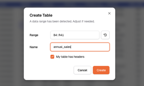
Click Create
Done. Your data is now a table with filtering ready to go.
What You Can Do
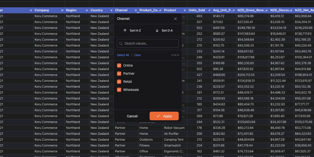
Filter and Sort
Click the dropdown arrow in any column header:
| Option | What it does |
|---|---|
| Sort A to Z | Sort smallest to largest (or A to Z) |
| Sort Z to A | Sort largest to smallest (or Z to A) |
| Filter by value | Show only rows that match |
| Clear filter | Show all rows again |
The dropdown icon changes when a filter is active so you know which columns are filtered.
Banded Rows
Tables automatically alternate row colors. This makes it easier to read across wide tables. You can turn this off in table properties.
Change the Style
- Click anywhere in the table
- Go to Format → Table Styles
- Pick a style from the gallery
Styles come in three categories:
- Light — Subtle, minimal
- Medium — Balanced colors
- Dark — Bold headers, high contrast
Use Column Names in Formulas
Tables let you use column names instead of cell addresses. This is called a “structured reference.”
Instead of =SUM(B2:B100), you write =SUM(Sales[Amount]). Much clearer.
The Syntax
| Reference | What it means | Example |
|---|---|---|
Table1[Column] | A whole column | =SUM(Sales[Amount]) |
[@Column] | This row’s value in that column | =[@Price]*[@Quantity] |
Table1[[Col1]:[Col2]] | Multiple columns | =SUM(Sales[[Q1]:[Q4]]) |
Table1[#Data] | All data rows (no headers) | — |
Table1[#Headers] | Just the header row | — |
Table1[#Totals] | Just the totals row | — |
Examples
Add up a column:
=SUM(Sales[Amount])Multiply two columns in the same row:
=[@Price] * [@Quantity]Use a table from outside it:
=AVERAGE(Inventory[Stock Level])As you type, column names appear in autocomplete. Press Tab to insert them.
Add a Total Row
Show sums, averages, or counts at the bottom of your table.
Click in the table
Click anywhere inside your table.
Turn on totals
Go to Table → Toggle Total Row.
Pick a function
Click the dropdown in each total cell to choose what to calculate.
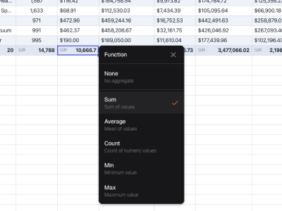
Available Functions
| Function | What it does |
|---|---|
| Sum | Add all values |
| Average | Get the mean |
| Count | Count how many values |
| Max | Find the largest |
| Min | Find the smallest |
| None | Show nothing |
Managing Tables
Add New Rows
Type in the row just below your table. It expands automatically. Formulas update too.
Resize Manually
Drag the handle in the bottom-right corner to grow or shrink the table.
Convert Back to Regular Cells
- Click in the table
- Go to Table → Convert to Range
This removes filters and column-name formulas. Your data and formatting stay.
Change Table Settings
Click in the table and open Table menu to:
- Rename the table
- Show or hide the header row
- Show or hide the total row
- Turn banded rows on or off
- Change the style
Tips
- Name your tables well — Change “Table1” to something like “SalesData”
- Keep column names short — Shorter names are easier to use in formulas
- Leave space between tables — One empty row or column is enough
- Use column names in formulas — They’re clearer than cell addresses and update automatically